BioMEMS

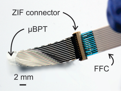
I spent two years in USC Biomedical Microsystems Laboratory working as an undergraduate researcher. One of the projects aims to treat hydrocephalus via a novel pressure sensor.¹

Keywords: pressure sensor, image processing, BioMEMS, implantable device, microbubble, fluid dynamics, device characterization, Boyle’s law.

Introducing a pressure sensor

Hydrocephalus occurs when excessive cerebrospinal fluid accumulates in the brain, which results in an abnormal widening of spaces. Since fluid accumulation poses potentially life-threatening pressure against brain tissues, it is necessary to monitor pressure chronically to drive timely therapeutic interventions. Hence, a new, flexible, MEMS-based, low-powered, biocompatible pressure sensor was being developed. This pressure sensor enables reliable sensing for chronic in-vivo implantation and provides immediate access to actionable pressure data. My job is to characterize the transducer’s design to maximize its sensitivity. So how does it work?

Principle of pressure sensing using a microbubble

The key idea of the design exploits how microbubbles respond instantaneously to external pressure variations. By isolating the microbubble in a microchannel filled with an electrolyte solution, we are able to mimic the wet, in-vivo environment of cerebrospinal fluid in hydrocephalus. Our goal is to infer pressure change by monitoring the behavior of the bubble dissolution.

Boyle’s law tells us that pressure of a gas is inversely related to its volume (\(P \varpropto \frac{1}{V}\)). Henry’s law tells us bubble dissolution rate linearly corresponds to change in pressure.

A microchannel is carefully fabricated into the device. The channel is connected with four electrodes: two on each side to measure the electrochemical differences (e.g. impedance) and two in the middle to generate a microbubble.

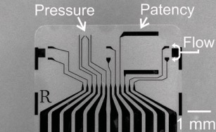
We first completely fill the microchannel with phosphate buffered saline (PBS) to mimic a wet, in-vivo environment. By a current-induced electrolysis from the nuclear cores, we create a microbubble from the middle of the channel.

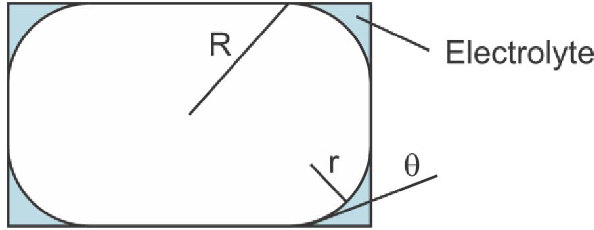
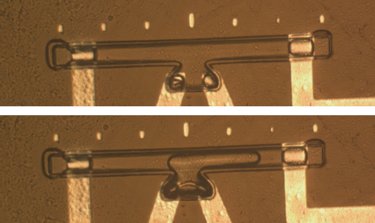
When a microbubble is trapped within a filled chamber with rectangular cross section, the gas tends to fill the middle of the cross sectional area and leave pockets of liquid at the corners. These capillaries allow an ionic conduction path within the channel.²

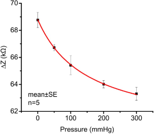
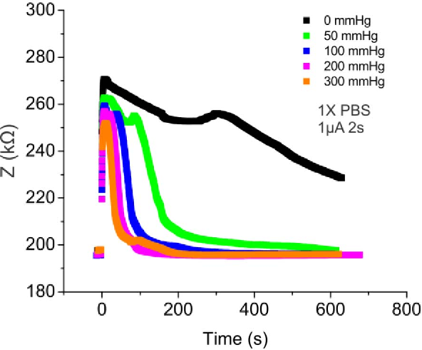
One electrochemical characterization we do is to chronically measure changes in impedance conducted through the liquid capillaries at the corners.² Though it is a good indicator of pressure change, a big obstacle we discover is the instability in impedance measurement from the microbubble generation. So we explore alternative ways to characterize microbubble behavior other than the established method of measuring impedance.

Bubble length tracking

In response to a pressure change, bubble length is more likely to vary than the cross section area in a microchannel.³ So can we infer pressure through tracking microbubble length, rather than using impedance measurements? With some simple image processing on the bubble snapshots taken 2 frames per second, we implement a Matlab program that automatically tracks changes of the microbubble volume in response to pressure.

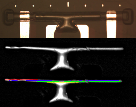
We take the raw, cropped, straightened image of the microchannel and subtract it from the initial image taken before a bubble is injected. By processing it into a B/W image of the isolated bubble, we then implement a program to track both ends of the bubble. Note that the markers on top of the channel are 100µm apart. They provide us a nice basis to measure the actual bubble length.

If you’re interested in the actual code, click open the collapsible:

    % iternate for the whole set of images
    files = dir(fullfile(mydir, 'img*.jpg'));
    first = 'img.jpg';
    count = 0;
    for file = files'
        fname = file.name;
        disp(fname);
        count = count + 1;
    % only start processing after the first image (the 'base' image)
        if (strcmp(fname,first))
            base = imread(fullfile(mydir, fname),'jpg');
            base = rgb2gray(base);
            basecropped = imcrop(base,crop_parameter);
            basecropped = imrotate(basecropped,angle,'bilinear','crop');
        else
            im = imread(fullfile(mydir, fname),'jpg');
            im = rgb2gray(im);
            imcropped = imcrop(im,crop_parameter);
            imcropped = imrotate(imcropped,angle,'bilinear','crop');
    % Subtract from the initial 'base' image that has no bubble
            diff = (imcropped - basecropped);
            diff = imadjust(diff);
    % ensure we get the correct length by measuring multiple rows
            for i = 0:2:test_rows
                [row,col] = find(diff(i+starting_row,:) > cut_off_pixel);
                [row5,col5] = find(diff(i+starting_row+5,:) > cut_off_pixel);
                [row10,col10] = find(diff(i+starting_row+10,:) > cut_off_pixel);
                [row15,col15] = find(diff(i+starting_row+15,:) > cut_off_pixel);
                combcol = union(col,col5);
                combcol = union(combcol,col10);
                combcol = union(combcol,col15);
                if(isempty(combcol))
                    bubble_length_ratio = [bubble_length_ratio;0];
                else
                    bubble_length = combcol(end)-combcol(1);
    % sometimes the the image is fuzzy or not cropped properly
                    continuous = bubble_length/(size(combcol,2)-size(combcol,1));
                    if(continuous < 1.5)
                        bubble_length_ratio = [bubble_length_ratio;bubble_length/base_length];
                    else
                        bubble_length_ratio = [bubble_length_ratio;0];
                    end
                end
            end
            bubble_length_array = [bubble_length_array, bubble_length_ratio];
            [max_ratio,max_row] = max(bubble_length_ratio);
            max_ratio
            max_row = starting_row + max_row;
            max_ratio_array = [max_ratio_array, max_ratio];
    %displaying images
            [row,col] = find(diff(max_row,:) > cut_off_pixel);
            [row5,col5] = find(diff(max_row+5,:) > cut_off_pixel);
            [row10,col10] = find(diff(max_row+10,:) > cut_off_pixel);
            [row15,col15] = find(diff(max_row+15,:) > cut_off_pixel);
            if(disp_images && count-1>=starting_image && count-1<=ending_image)
                figure
                imshow(diff);
                title(num2str(fname));
                hold on;
                if(~isempty(col))
                    plot(col,max_row,'rx', 'MarkerSize', 5);
                end
                if(~isempty(col5))
                    plot(col5,max_row+5,'bx', 'MarkerSize', 5);
                end
                if(~isempty(col10))
                    plot(col10,max_row+10,'gx', 'MarkerSize', 5);
                end
                if(~isempty(col15))
                    plot(col15,max_row+15,'yx', 'MarkerSize', 5);
                end
                pause(.2);
            end
            bubble_length_ratio = [];
        end
    end
    

Results

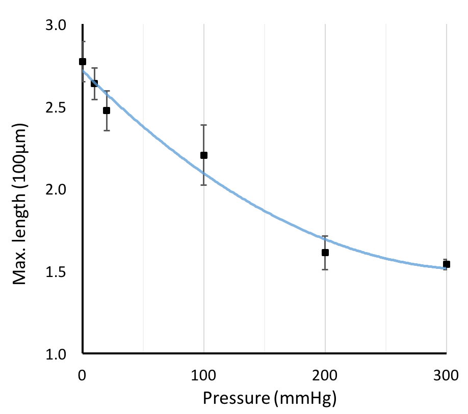
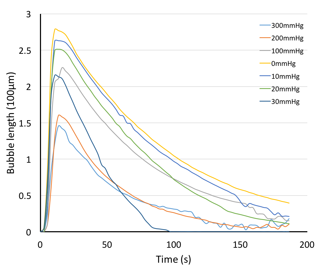
If we compare the bubble length results to the impedance measurements⁴, we can see some similarities. Both bubble length and impedance measurements show us their inverse relationships with pressure, and can capture the essence of the microbubble behavior inside the channel in a similar fashion.

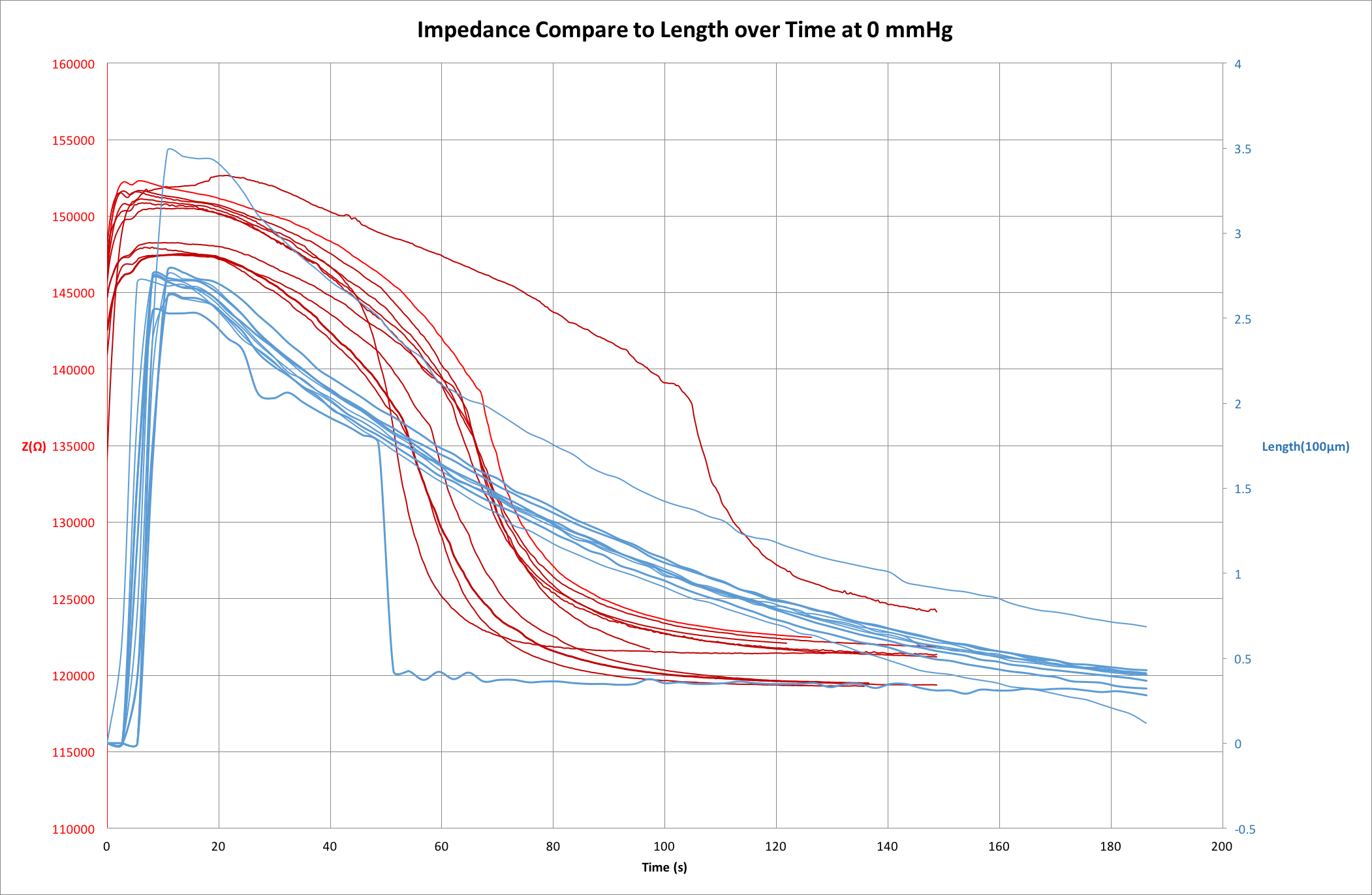
We have shown microbubble length tracking is a nice and intuitive visual tool for us to monitor bubble dissolution. However, there is one issue remains unsolved - we couldn’t quite explain the correlations between the two indicators (bubble length and impedance). If we plot the two measurements overlapping each other, as the bubble dissolves, the two measurements appear to have different curves as the bubble dissolves.⁵

Conclusion

Impedance measurements remain to be a precise benchmark for our device characterization, but this project provides us an alternative visual indicator of the device performance. It can be especially useful when the electrochemical performance is unstable/unreliable for some devices.