Feature Reuse with ANIL
In this article, we will dive into a meta-learning algorithm called ANIL (Almost No Inner Loop) presented by Raghu et al., 2019, and explain how to implement it with learn2learn.

Original published on learn2learn.net, this tutorial is written for experienced PyTorch users who are getting started with meta-learning.
Overview
- We look into how ANIL takes advantage of feature reuse for few-shot learning.
- ANIL simplifies MAML by removing the inner loop for all but the task-specific head of the underlying neural network.
- ANIL performs as well as MAML on benchmark few-shot classification and reinforcement learning tasks, and is computationally more efficient than MAML.
- We implement ANIL with learn2learn and provide additional results of how ANIL performs on other datasets.
- Lastly, we explain the implementation code step-be-step, making it easy for users to try ANIL on other datasets.
ANIL algorithm
Among various meta-learning algorithms for few-shot learning, MAML (model-agnostic meta-learning) (Finn et al. 2017) has been highly popular due to its substantial performance on several benchmarks. Its idea is to establish a meta-learner that seeks an initialization useful for fast learning of different tasks, then adapt to specific tasks quickly (within a few steps) and efficiently (with only a few examples). There are two types of parameter updates: the outer loop and the inner loop. The outer loop updates the meta-initialization of the neural network parameters to a setting that enables fast adaptation to new tasks. The inner loop takes the outer loop initialization and performs task-specific adaptation over a few labeled samples. To read more about meta-learning and MAML, you can read the summary article written by Finn on learning to learn and Lilian Weng’s review on meta-learning.
In 2019, Raghu et al. conjectured that we can obtain the same rapid learning performance of MAML solely through feature reuse. To test this hypothesis, they introduced ANIL (almost no inner loop), a simplified algorithm of MAML that is equally effective but computationally faster.
Rapid learning vs. feature reuse
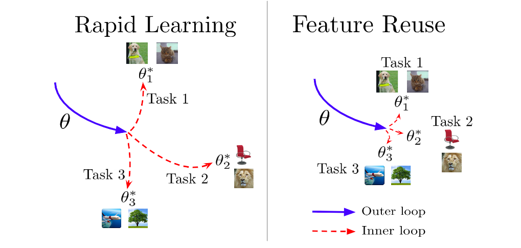
Before we describe ANIL, we have to understand the difference between rapid learning and feature reuse. In rapid learning, the meta-initialization in the outer loop results in a parameter setting that is favorable for fast learning, thus significant adaptation to new tasks can rapidly take place in the inner loop. In feature reuse, the meta-initialization already contains useful features that can be reused, so little adaptation on the parameters is required in the inner loop. To prove feature reuse is a competitive alternative to rapid learning in MAML, the authors proposed a simplified algorithm, ANIL, where the inner loop is removed for all but the task-specific head of the underlying neural network during training and testing.
ANIL vs. MAML
Now, let us illustrate the difference mathematically. Let \(\theta\) be the set of meta-initialization parameters for the feature extractable layers of the network and \(w\) be the meta-initialization parameters for the head. We obtain the label prediction \(\hat{y} = w^T\phi_\theta(x)\), where x is the input data and \(\phi\) is a feature extractor parametrized by \(\theta\).
Given \(\theta_i\) and \(w_i\) at iteration step \(i\), the outer loop updates both parameters via gradient descent:
\[\theta_{i+1} = \theta_i - \alpha\nabla_{\theta_i}\mathcal{L}_{\tau}(w^{\prime \top}_i\phi_{\theta^\prime_i}(x), y)\] \[w_{i+1} = w_i - \alpha\nabla_{w_i}\mathcal{L}_{\tau}(w^{\prime \top}_i\phi_{\theta^\prime_i}(x), y)\]where \(\mathcal{L}_\tau\) is the loss computed for task \(\tau\), and \(\alpha\) is the meta learning rate in the outer loop. Notice how the gradient is taken with respect to the initialization parameters \(w_i\) and \(\theta_i\), but the loss is computed on the adapted parameters \(\theta_i^\prime\) and \(w_i^\prime\). For one adaptation step in the inner loop, ANIL computes those adapted parameters as:
\[\theta_{i}^\prime = \theta_i\] \[w_{i}^\prime = w_i - \beta\nabla_{w_i}\mathcal{L}_{\tau}(w_i^T\phi_{\theta_i}(x), y)\]where \(\beta\) is the learning rate of the inner loop.
Concretely, ANIL keeps the feature extractor constant and only adapts the head with gradient descent.
In contrast, MAML updates both the head and the feature extractor:
\[\theta_{i}^\prime = \theta_i - \beta\nabla_{\theta_i}\mathcal{L}_{\tau}(w_i^T\phi_{\theta_i}(x), y)\] \[w_{i}^\prime = w_i - \beta\nabla_{w_i}\mathcal{L}_{\tau}(w_i^T\phi_{\theta_i}(x), y).\]Unsurprisingly, ANIL is much more computationally efficient since it requires fewer updates in the inner loop. What might be surprising, is that this efficiency comes at almost no cost in terms of performance.
Results
ANIL provides fast adaptation in the absence of almost all inner loop parameter updates, while still matching the performance of MAML on few-shot image classification with Mini-ImageNet and Omniglot and standard reinforcement learning tasks.
| Method | Omniglot-20way-1shot | Omniglot-20way-5shot | Mini-ImageNet-5way-1shot | Mini-ImageNet-5way-5shot |
|---|---|---|---|---|
| MAML | 93.7 ± 0.7 | 96.4 ± 0.1 | 46.9 ± 0.2 | 63.1 ± 0.4 |
| ANIL | 96.2 ± 0.5 | 98.0 ± 0.3 | 46.7 ± 0.4 | 61.5 ± 0.5 |
Using ANIL with learn2learn
With our understanding of how ANIL works, we are ready to implement the algorithm. An example implementation on the FC100 dataset is available at: anil_fc100.py. Using this implementation, we are able to obtain the following results on datasets such as Mini-ImageNet, CIFAR-FS and FC100 as well.
| Dataset | Architecture | Ways | Shots | Original | learn2learn |
|---|---|---|---|---|---|
| Mini-ImageNet | CNN | 5 | 5 | 61.5% | 63.2% |
| CIFAR-FS | CNN | 5 | 5 | n/a | 68.3% |
| FC100 | CNN | 5 | 5 | n/a | 47.6% |
ANIL Implementation
This section breaks down step-by-step the ANIL implementation with our example code.
Creating dataset
train_dataset = l2l.vision.datasets.FC100(root='~/data',
                                          transform=tv.transforms.ToTensor(),
                                          mode='train')
train_dataset = l2l.data.MetaDataset(train_dataset)
First, data are obtained and separated into train, validation and test dataset with l2l.vision.datasets.FC100. tv.transforms.ToTensor() converts Python Imaging Library (PIL) images to PyTorch tensors. l2l.data.MetaDataset is a thin wrapper around torch datasets that automatically generates bookkeeping information to create new tasks.
train_transforms = [
    FusedNWaysKShots(train_dataset, n=ways, k=2*shots),
    LoadData(train_dataset),
    RemapLabels(train_dataset),
    ConsecutiveLabels(train_dataset),
]
train_tasks = l2l.data.TaskDataset(train_dataset,
                                   task_transforms=train_transforms,
                                   num_tasks=20000)
l2l.data.TaskDataset creates a set of tasks from the MetaDataset using a list of task transformations:
-
FusedNWaysKShots(dataset, n=ways, k=2*shots): efficient implementation to keep \(k\) data samples from \(n\) randomly sampled labels. The number of samples \(k\) is twice the number of shots because one half of the samples are for adaption and the other half are for evaluation in the inner loop. LoadData(dataset): loads a sample from the dataset given its index.RemapLabels(dataset): given samples from \(n\) classes, maps the labels to \(0, \dots, n\).ConsecutiveLabels(dataset): re-orders the samples in the task description such that they are sorted in consecutive order.
For more details, please refer to the documentation of learn2learn.data.
Creating model
features = l2l.vision.models.ConvBase(output_size=64, channels=3, max_pool=True)
features = torch.nn.Sequential(features, Lambda(lambda x: x.view(-1, 256)))
features.to(device)
head = torch.nn.Linear(256, ways)
head = l2l.algorithms.MAML(head, lr=fast_lr)
head.to(device)
We then instantiate two modules, one for features and one for the head. ConvBase instantiates a four-layer CNN, and the head is a fully connected layer. Because we are not updating the feature extractor parameters, we only need to wrap the head with the l2l.algorithms.MAML() wrapper, which takes in the fast adaptation learning rate fast_lr used for the inner loop later.
For more details on the MAML wrapper, please refer to the documentation of l2l.algorithms.
Optimization setup
all_parameters = list(features.parameters()) + list(head.parameters())
optimizer = torch.optim.Adam(all_parameters, lr=meta_lr)
loss = nn.CrossEntropyLoss(reduction='mean')
Next, we set up the optimizer with mini-batch SGD using torch.optim.Adam, which takes in both feature and head parameters, and learning rate meta_lr used for the outer loop.
Outer loop
for iteration in range(iters):
    ...
    for task in range(meta_bsz):
        learner = head.clone()
        batch = train_tasks.sample()
        ...
For training, validation and testing, we first sample a task, then copy the head with head.clone(), which is a method exposed by the MAML wrapper for PyTorch modules, akin to tensor.clone() for PyTorch tensors. Calling clone() allows us to update the parameters of the clone while maintaining ability to back-propagate to the parameters in head. There’s no need for feature.clone() as we are only adapting the head.
Inner loop
def fast_adapt(batch, learner, features, loss, adaptation_steps, shots,
               ways, device=None):
    data, labels = batch
    data, labels = data.to(device), labels.to(device)
    data = features(data)

    # Separate data into adaptation/evaluation sets
    adaptation_indices = np.zeros(data.size(0), dtype=bool)
    adaptation_indices[np.arange(shots*ways) * 2] = True
    evaluation_indices = torch.from_numpy(~adaptation_indices)
    adaptation_indices = torch.from_numpy(adaptation_indices)
    adaptation_data, adaptation_labels = data[adaptation_indices], labels[adaptation_indices]
    evaluation_data, evaluation_labels = data[evaluation_indices], labels[evaluation_indices]

    for step in range(adaptation_steps):
        train_error = loss(learner(adaptation_data), adaptation_labels)
        learner.adapt(train_error)

    predictions = learner(evaluation_data)
    valid_error = loss(predictions, evaluation_labels)
    valid_accuracy = accuracy(predictions, evaluation_labels)
    return valid_error, valid_accuracy
In fast_adapt(), we separate data into adaptation and evaluation sets with k shot samples each. In each adaptation step, learner.adapt() takes a gradient step on the loss and updates the cloned parameter, learner, such that we can back-propagate through the adaptation step. Under the hood, this is achieved by calling torch.autograd.grad() and setting create_graph=True. fast_adapt() then returns the evaluation loss and accuracy based on the predicted and true labels.
Some may ask, why is the number of adaptation steps so small? To demonstrate fast adaptation, we want the algorithm to adapt to each specific task quickly within a few steps. Since the number of samples is so small in few-shot learning, increasing number of adaptation steps would not help raising the performance.
Closing the outer loop
evaluation_error.backward()
meta_train_error += evaluation_error.item()
meta_train_accuracy += evaluation_accuracy.item()
...
# Average the accumulated gradients and optimize
for p in all_parameters:
    p.grad.data.mul_(1.0 / meta_bsz)
optimizer.step()
We compute the gradients with evaluation_error.backward() right after the inner loop updates to free activation and adaptation buffers from memory as early as possible. Lastly, after collecting the gradients, we average the accumulated gradients and updates the parameter at the end of each iteration with optimizer.step().
Conclusion
Having explained the inner-workings of ANIL and its code implementation with learn2learn, I hope this tutorial will be helpful to those who are interested in using ANIL for their own research and applications.
References
- Raghu, A., Raghu, M., Bengio, S., & Vinyals, O. (2019). Rapid Learning or Feature Reuse? Towards Understanding the Effectiveness of MAML. arXiv. http://arxiv.org/abs/1909.09157
- Finn, C., Abbeel, P., & Levine, S. (2017). Model-Agnostic Meta-Learning for Fast Adaptation of Deep Networks. arXiv. http://arxiv.org/abs/1703.03400