Cosine Tuning in Motor Cortical Neurons
Cosine tuning has been observed in most neurons in motor systems including human and non-human primate. This article serves as an introduction to this topic mainly through understanding the paper that first reported it in 1982 1. This early work has inspired a number of successful algorithms for decoding neural activity in motor cortex to perform offline reconstruction or online control of cursors or robotic arms.
Goals
- Are there any relations of single neuron activity to the direction of movement?
- Can we quantify the relations with a distribution?
- How do we fit cosine tuning?
- What is the biological significance of cosine tuning?
A brief history
In 1968, Evarts first observed the activity of single cells in the motor cortex of the monkey performing push-pull movements. He made pioneer discovery on relating cortical cells in the arm-related area to the movements and the muscular force generated by the animal.
Neuronal activity in the primate motor cortex can be related to the force exerted, the direction, or the velocity of the movement, alone or in combination. Of the three, the relations to the direction of the movement have been least well analyzed.
Previous studies utilized only two opposite directions in their experiments. So in 1982, Georgopoulos and colleagues designed an 8-direction reach task to examine the relations of single neuron activity to the direction of movement.
Experimental setup
Four rhesus monkeys were used in Georgopoulos’s experiment. On the working surface were eight peripheral targets arranged equidistantly on the circumference circle and a target at the center of the circle. The monkeys were trained to perform a reach task to move a freely moveable manipulandum from the center to one of the eight directions of the working surface, prompted when the LED lights up randomly at one of the eight targets. The eight direction of the movement trajectories covered the whole circle at intervals of 45\(^{\circ}\). This classical setup is later referred to a center-out or radial-8 task.
Neural data were collected through placing a recording chamber over the arm area of the motor cortex under general anesthesia.
Analysis using first degree periodic (sinusoidal) regression
The following expressions are extracted from their paper.
Let \(y_i (i = 1, 2, ..., 8 )\) be the mean rate when a cell discharges during movements towards direction \(\theta_i = 0, 45, 90, ..., 315^{\circ}\), respectively. We can fit a regress with
\[y = b_0 + b_1 \cos \theta + b_2 \sin \theta\]or alternatively,
\[y = b_0 + \sqrt{b^2_1 + b^2_2} \cos (\theta - \theta_0)\]where \(b_0, b_1, b_2\) are regression coefficients that can be estimated with least square unbiased estimators as follow
\[b_0 = \bar{y} = 1/8(y_1 + y_2 + y_3 + ... + y_8)\] \[b_1 = 1/4\big[\frac{1}{\sqrt{2}}(y_2 + y_4 - y_6 - y_8) + (y_3- y_7)\big]\] \[b_2 = 1/4\big[\frac{1}{\sqrt{2}}(y_2 - y_4 - y_6 + y_8) + (y_1- y_5)\big]\]\(\theta_0\) is the preferred direction. Using trigonometric moments, we can calculate \(\theta_0\) by first defining
\[\theta_0' = \tan^{-1}(\frac{b_2}{b_1}), \quad -45^{\circ} < \theta_0' < 45^{\circ}\]According to the quadrant, \(\theta_0\) is given by
\[\theta_0 = \theta_0' \qquad\qquad\qquad \ if \ \ b_1 > 0, b_2 > 0\] \[\theta_0 = \theta_0' + 180^{\circ} \qquad\quad if \ \ b_2 < 0\] \[\theta_0 = \theta_0' + 360^{\circ} \qquad\quad if \ \ b_1 < 0, b_2 > 0\]A performance measure \(R^2\) can indicate how well the regression fits:
\[R^2 = \frac{\sum\hat{y}^{2}}{\sum{y^{2}}} = \frac{4(b^2_1+b^2_2)}{\sum{(y-\bar{y})^2}}\]An index of the directional modulation for increase in discharge at the preferred direction over the overall mean can be expressed as
\[I = \frac{\sqrt{b^2_1 + b^2_2}}{b_0}, \quad b_0 > 0\]Results from the paper
Of the 606 arm-related cells tested, 323 cells were active under the task circumstances. 296 cells had significant correlations between cell discharge and the direction of movement during the total experimental time. Below are some of the key findings.
-
Directional tuning curve: 241 cells, about 80% of the total, expressed a directional preference and 75 \(\%\) of them has an adequate fit with R\(^2 \geq\) 0.7. More cells preferred direction of 45\(^{\circ}\) than 225\(^{\circ}\).
-
Change of neural discharge: when the movement direction was near (further away) the cell’s preferred direction, an increase in activity occurred more (less) frequently.
-
cells with preferred directions at or near (opposite or far from) the direction of the upcoming movement will be activated (inhibited).
Biological Significance of Cosine Tuning
Georgopoulos and colleagues were the first to present that neurons in the arm-related area in motor cortex exhibit preferred directions through a center-out task and can be fitted by cosine tuning regression. From a biological perspective, Todorov provided insight into as of why cosine tuning can be significant. Also through empirical observations, he concluded that the cosine tuning minimizes the net effect of neuromotor noise, thereby minimizing expected errors in force production2. He showed that cosine curve is the optimal force activation profile under arbitrary dimensions and arbitrary force direction distribution.
Working example
Let’s apply the regression on a simulated dataset.
% Simulating a simple dataset
targets = 45 * (0:8);
y = [-0.1900  -0.1936  0.2676  0.2650  0.2424 -0.0260 -0.2355 -0.2910];
err = [0.0600  0.0703  0.0959  0.0989  0.0495  0.1356  0.0813  0.0804];

% fit a cosine function
[b0, b1, b2, theta0, R, I] = CosineTuningRegression(y);
angles = linspace(0, 2 * pi, 360);
yreg1 = b0 + b1 * sin(angles) + b2 * cos(angles);
yreg2 = b0 + sqrt(b1^2 + b2^2) * cos(angles - theta0); % the same with yreg1

% plot fitted curve
y = [y, y(1)];
err = [err, err(1)]; % same data point at 0 and 360 degree
figure
plot(angles * 180/pi, yreg1);
hold on
scatter(targets, y, 14, 'filled', 'k');
errorbar(targets, y, err, 'k', 'LineStyle', 'none');
xlabel('Angle', 'fontsize', 14);
xticks(targets)
axis([0, 360, -1, 1]);
legend('regression fit', 'y', 'error', 'fontsize', 14)
text(280, 0.5, ['R^2 = ',num2str(R)], 'fontsize', 14)
box off

function [b0, b1, b2, theta0, R, I] = CosineTuningRegression(y)
    [ny, ly] = size(y);
    if(ly > ny); y = y'; end
    [ny, ly] = size(y);
    if(ny~=8); error('The input vector should contain only 8 directions.');end
    if(ly~=1); error('Only one channel should be calculated each time');end
    b0 = mean(y);
    b1 = ((y(2) + y(4) - y(6) - y(8)) / sqrt(2) + (y(3) - y(7))) / 4;
    b2 = ((y(2) - y(4) - y(6) + y(8)) / sqrt(2) + (y(1) - y(5))) / 4;
    theta0 = atan2(b1, b2);
    R = 4 * (b1^2 + b2^2) / sum((y - b0).^2);
    I = sqrt(b1^2 + b2^2) / b0;
end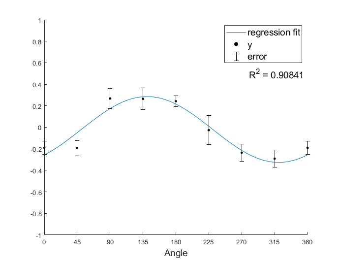
-
A. P. Georgopoulos, J. F. Kalaska: R. Caminiti, and J. T. Massey. “on The Relations Between The Direction Of Two-dimensional Arm Movements And Cell Discharge In Primate Motor Cortex.” The Journal of Neuroscience, Vol. 2, No. 11, pp. 1527-1537. 1982 ↩
-
E. Todorov. 2002. “Cosine Tuning Minimizes Motor Errors.” Neural Computation 14 (6): 1233–60. ↩