SubID simulations
Adaptive subspace identification algorithm for dynamic tracking
On this page, I will go over what I wrote on my senior thesis. I only extract key research ideas and figures from my thesis. To view the full version of my senior thesis, click here. To view the matlab code, please go to my github repo.
Keywords: adaptive subspace identification, dynamic tracking, state-space models, forgetting factor, prediction error, tracking error.
Introduction
Through identifying and tracking of brain network dynamics, neuroscientists have been able to understand neural mechanisms in a deeper level for the past decades. A broad range of neurological disorders can be effectively treated by developing adaptive closed-loop stimulation therapies or brain-machine-interface (BMI). They utilize real-time neural signal monitoring and brain states control using electrical stimulation. However, due to the non-stationary and time-variant properties of some brain network dynamics, such modeling becomes challenging.
In this work, we implement an adaptive subspace identification algorithm (subID) developed by yang et. al.1 and test it on simulated time-invariant and time-varying state-space models (SSMs). We run some simulations to prove that the algorithm can track the poles trajectories of the time-varying State-space models in an adaptive manner with high accuracy. By quantifying the performance with prediction error and tracking error, we experimentally show that the proposed adaptive identification algorithm could better predict and track poles of the true time-varying system, as compared to the traditional non-adaptive identification algorithm.
Adaptive algorithm
Disclaimer: I try to keep the explanation of this section brief. For details of the subID algorithm, experimental setup, training and testing, performance measures, please refer to my thesis.
We first formulate time-varying SSMs of purely stochastic systems as
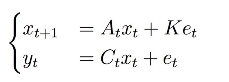
where \(x\) is the hidden state, \(y\) is the observation state, \(A\) and \(C\) are time-varying system matrices, \(K\) is the forward Kalman gain, \(e_t\) is a noise set to zero mean with variance of 0.0001. In our experiments, we set our system to a second order with zero inputs and two outputs. \(A\) is the only time-varying matrix with changing diagonal elements in each time steps, with absolute value of all poles of \(A\) less than 1 (stability requirement). The \(C\) matrix is set to an identity matrix.
We adapt our adaptive subID algorithm from the original time-invariant subID algorithm from Overschee’s book (a good introduction to subID)2. To make the algorithm adaptive, we introduce a user-defined forgetting factor, β, to estimate time-varying output covariance matrices,1
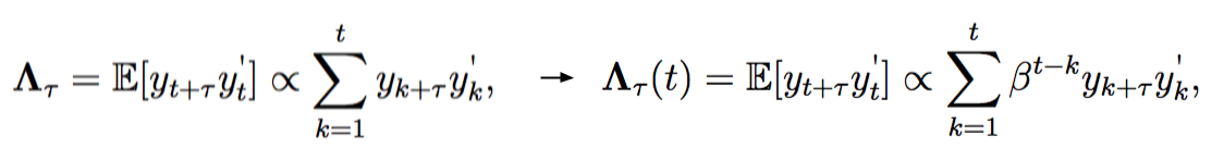
Here, we update the estimate of output covariance matrices at each time step, while putting more weight on the recent data than past data. A small β implies the recent data are more heavily weighted, and a large β implies the past data are weighted almost as heavy as the recent data. β = 1 means that the entire dataset is weighted equally, which is equivalent to the non-adaptive output covariance matrices.
Since we calculate new output covariance matrices using QR-decomposition, and that they are updated at every time step, we need to recalculate QR matrices at every time step. To enable an efficient, online operation of the QR-decomposition, we use a recursive algorithm to update the R matrix in the QR-decomposition 1 with the help of Givens rotation (check out qrinsert.m in Matlab). I will leave the math details in my thesis.
Training and testing sets
We allocate the 5500 time steps into 5000 for training and 500 for testing. The adaptive algorithm estimates the SSM at each time step of the training set. During training, we record the estimated poles of the time varying system at each time step to investigate the pole tracking ability of the algorithm. We fix SSM_adpt at the last estimate. The non-adaptive algorithm uses the entire training data to produce a single estimation, SSM_non-adpt. Using SSM_adpt and SSM_non-adpt, we evaluate the prediction power on the testing set, which is unseen by both algorithms. We do not further adapt the SSM_adpt during testing. We compare these predictions to the baseline, which is defined as the true SSM at the last time step of the training set.
Performance measures
We introduce two error metrics to evaluate the algorithm’s performance. We quantify 1) a prediction error (PE), using a normalized root mean square error between the predicted outputs and the true outputs in the test set, and 2) a tracking error (TE), also using a normalized root mean square error between an averaged estimated and the true eigenvalues of the TV matrix at each time step.
One thing to note is that we take the mean and standard error of the mean (SEM) of PE of all 200 Monte Carlo simulations, but we perform TE on the averaged pole trajectories over all Monte Carlo simulations, instead of on individual simulations, which have estimated poles with very large variance. We then take the mean and SEM of TE across all poles. The exact equations of the error metrics are in my thesis.
Results
For each case, we visually evaluate the pole tracking ability of the adaptive algorithm and compare the output estimation in the test set. We also quantitatively compare PE and TE of both algorithms.

Time-invariant system
_eig_test_enlarged.png)

Since this is a time-invariant system, we set β = 1 to show that the adaptive algorithm can perform equally well when all past data are used. The pole estimation using the non-adaptive algorithm can perfectly track the true time-invariant poles and the estimated poles using adaptive algorithm can converge quickly to the true poles as well.
Time-varying systems
-eig-99.png)
-test-99.png)
-eig-99.png)
-test-99.png)
-eig-99.png)
-test-99.png)
-eig-99.png)
-test-99.png)
For all time-varying cases, we can point out that the non-adaptive algorithm fails to track the poles trajectories over time. Even when the non-adaptive algorithm uses all past data, since only one estimated system is produced, it is impossible to track poles in an adaptive manner. On the other hand, the adaptive algorithm can effectively track the true poles of the time-varying system. In figure (b), the estimated outputs of the test set using the adaptive algorithm are also closer to the true outputs compared to the non-adaptive algorithm. Judging visually, we can already conclude that the adaptive algorithm has a higher estimation power in the simulated time-varying cases.
Simulations summary
We also want to compare the algorithms quantitatively using our defined error measures. For all time-varying cases, we obtain TE_adpt < TE_non-adpt and PE_baseline < PE_adpt < PE_non-adpt, proving that the performance of the adaptive algorithm is indeed better than the non-adaptive algorithm. Meanwhile, adaptive algorithm can perform equally well as the non-adaptive algorithm in the time-invariant case.
| cases | TE_adpt | TE_non-adpt | PE_adpt | PE_non-adpt | PE_baseline |
|---|---|---|---|---|---|
| TI | 1.01±0.33% | 0.079±0.062% | 30.18±0.05% | 30.19±0.05% | 25.81±0.02% |
| random walk | 3.76±0.14% | 10.85±5.03% | 20.50±0.21% | 28.26±0.05% | 13.47±0.01% |
| linear | 1.96±0.13% | 6.96±0.70% | 15.85±0.19% | 19.77±0.05% | 11.10±0.001% |
| step-up | 2.68±0.75% | 14.48±0.35% | 13.36±0.17% | 15.23±0.04% | 9.59±0.001% |
| linear+ step-up | 3.78±0.05% | 7.06±0.75% | 17.80±0.19% | 20.77±0.05% | 13.70±0.002% |
Influence of the forgetting factor
One goal of the project is to determine the best value of the forgetting factor, β . The figure below displays the pole trajectories of some time-varying cases as β increase from 0.8 to 1. Remember, larger the value of β, heavier the past data are weighted. A β = 1 means that the entire dataset is weighted equally.
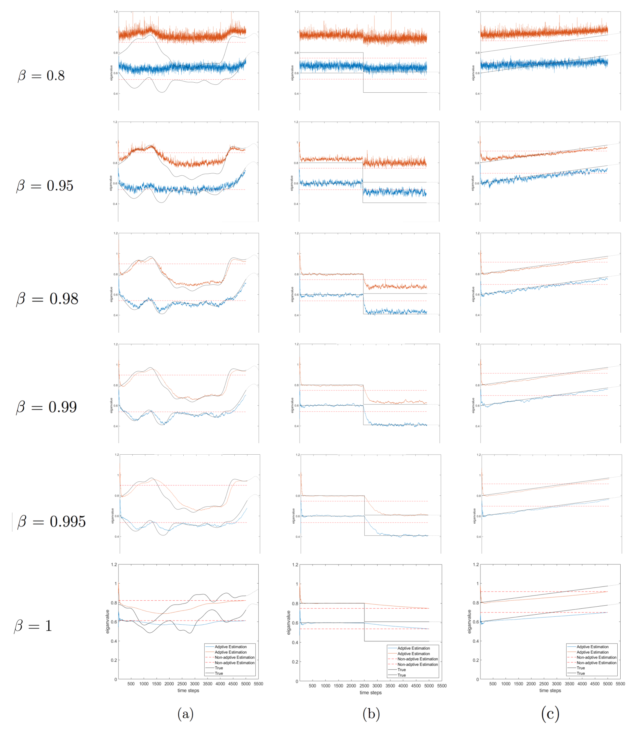
For β = 0.8, the pole trajectories of all cases are poorly estimated with large estimate variance. As the value of β increases from 0.8 to 0.98, the algorithm starts to perform more accurately in tracking poles. The estimate variance is also reduced as the value of β gets close to 1. When β = 1, the algorithm cannot track any time-varying part of the system in all cases, because the weights on past data equal to the weights on the recent data.
The performance of the algorithm with β = 0.98, 0.99, and 0.995 is very similar in terms of pole tracking, but there is a difference in terms of rate of convergence to the true poles. Closer the value of β to 1, more recent data are weighted in the algorithm, so longer it takes to converge to the true poles. As the value of β increases from 0.98 to 0.995, we can see an increasing delay in pole convergence in the random walk case and a slower convergence in the step function case. In real-life scenarios, maintaining a quick rate of convergence is surely something scientist concerns.
Additional Work
My thesis has more contents that I didn’t get to cover here. To be specific, we investigate the effect of the forgetting factor and training set length empirically (with error measures) to best optimize our simulations. I also encourage you to read the details of the algorithm in the method section.
-
Y. Yang, E. Chang, and M. Shanechi, “Dynamic tracking of non-stationarity in human ECoG activity,” Proc. IEEE Engineering in Medicine and Biology Society Conference(EMBC), Jeju Island, Korea, pp. 1660–1663, 2017. ↩ ↩2 ↩3
-
P. Overschee and B. Moor, Subspace Identification for Linear Systems: Theory, Implementation, Applications, vol. 3. Kluwer academic publishers Dordrecht, 1996. ↩